Documentation for pyIAST
This Python package, pyIAST, predicts mixed-gas adsorption isotherms from a set of pure-component gas adsorption isotherms in a nanoporous material using Ideal Adsorbed Solution Theory (IAST).
pyIAST characterizes a pure-component adsorption isotherm from a set of simulated or experimental data points by:
- fitting an analytical model to the data [e.g., Langmuir, quadratic, BET, Dual-site Langmuir, Henry’s law, approximated Temkin isotherm].
- linearly interpolating the data.
Then, pyIAST performs IAST calculations to predict the mixed-gas adsorption isotherms on the basis of these pure-component adsorption isotherm characterizations.
pyIAST can handle an arbitrary number of components.
Please see our article for theoretical details and consider citing our article if you used pyIAST in your research:
C. Simon, B. Smit, M. Haranczyk. pyIAST: Ideal Adsorbed Solution Theory (IAST) Python Package. Computer Physics Communications. (2015)
For example, consider that we have pure-component methane and ethane adsorption isotherms in metal-organic framework IRMOF-1 at 298 K, shown in Fig. 1.
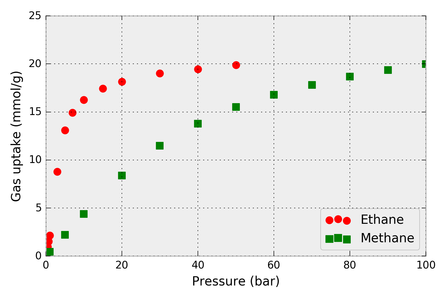
Figure 1. Pure-component methane and ethane adsorption isotherms – the amount of gas adsorbed as a function of pressure– in metal-organic framework IRMOF-1. Simulated data.
Using the pure-component isotherm data in Fig. 1, pyIAST can predict the methane and ethane uptake in IRMOF-1 in the presence of a mixture of ethane and methane at 298 K under a variety of compositions. For example, for a mixture at 65.0 bar, Fig. 2 shows that the mixed-gas adsorption isotherms in IRMOF-1 predicted by pyIAST (lines) agree with binary component Grand-canonical Monte Carlo simulations (points).
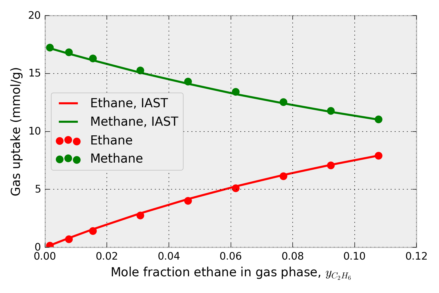
Figure 2. Methane and ethane adsorption in IRMOF-1 in the presence of a mixture of methane and ethane at 65.0 bar and 298 K. The x-axis shows the composition of ethane in the mixture. The data points are from binary grand-canonical Monte Carlo simulations; the lines are from pyIAST.
To ask a question, request an additional feature, report a bug, or suggest an improvement, submit an issue on Github or discuss on Gitter.
Installation
To install pyIAST, use the Python package manager pip:
sudo pip install pyiast
pyIAST runs on Python 3.x only (not Python 2.x).
As an alternative method to install pyIAST, clone the repository on Github. cd into the main directory pyIAST and run the setup.py script in the terminal:
sudo python setup.py install
If on Windows, run the setup file from a command prompt (Start –> Accessories):
setup.py install
New to Python?
If new to Python, I highly recommend working in the Jupyter Notebook; test scripts and tutorials for this code are written in Jupyter Notebooks. The instructions for getting started with Python for scientific computing are here.
pyIAST tutorial
For this tutorial on pyIAST, enter the /test directory of pyIAST. While you can type this code into the Python shell, I highly recommend instead opening a Jupyter Notebook.
First, import pyIAST into Python after installation.
import pyiast
For our tutorial, we have the pure-component methane and ethane adsorption isotherm data for metal-organic framework IRMOF-1 in Fig 1. We seek to predict the methane and ethane uptake in the presence of a binary mixture of methane and ethane in IRMOF-1 at the same temperature. As an example for this tutorial, we seek to predict the methane and ethane uptake of IRMOF-1 in the presence a 5/95 mol % ethane/methane mixture at a total pressure of 65.0 bar and 298 K.
Import the pure-component isotherm data
First, we load the pure-component isotherm data into Python so we can pass it into pyIAST. The data in Fig. 1 (from single component grand-canonical Monte Carlo simulations) are present in the CSV files:
- IRMOF-1_ethane_isotherm_298K.csv
- IRMOF-1_methane_isotherm_298K.csv
To import this data into Python, use the Pandas package (documentation for Pandas). The following code will return a Pandas DataFrame instance, which is useful for storing and manipulating tabular data.
import pandas as pd
df_ch4 = pd.read_csv("IRMOF-1_methane_isotherm_298K.csv")
df_ch3ch3 = pd.read_csv("IRMOF-1_ethane_isotherm_298K.csv")
You can check that your data has loaded correctly by looking at the head of the DataFrame:
df_ch4.head()
The units for pressure and loading in both DataFrames must be consistent; loading of gas must be in a molar quantity for IAST to apply (e.g. mmol/g or mmol/cm3). pyIAST will then work with these units throughout.
To load data into a Pandas DataFrame that is not in the CSV format, see the documentation for Pandas. Pandas is generally a very useful tool for manipulating data. See the 10 Minutes to pandas tutorial.
Construct pure-component isotherm objects
Next, we use pyIAST to translate the pure-component methane and ethane adsorption isotherm data into a model, which we will subsequently feed into pyIAST’s IAST calculator.
There are two different pure-component isotherm data characterizations in pyIAST:
- pyiast.ModelIsotherm
- pyiast.InterpolatorIsotherm
In the first, an analytical model (e.g. Langmuir) is fit to the data, and the isotherm thereafter is characterized by this fitted analytical model. In the second, pyIAST linearly interpolates the data and uses numerical quadrature to compute the spreading pressure, which is an integration involving the isotherm for IAST calculations.
Note that pyIAST allows you to mix isotherm models for an IAST calculation (e.g. use Langmuir for methane but interpolate for ethane).
For both ModelIsotherm and InterpolatorIsotherm, we construct the instance by passing the Pandas DataFrame with the pure-component adsorption isotherm data and the names of the columns that correspond to the loading and pressure.
ModelIsotherm
Here, in the construction of the instance of a ModelIsotherm, the data fitting to the analytical model is done under the hood. As an example, to construct a ModelIsotherm using the Langmuir adsorption model for methane (see Fig. 1), we pass the DataFrame df_ch4 and the names (keys) of the columns that correspond to the loading and pressure. In IRMOF-1_methane_isotherm_298K.csv, the name of the loading and pressure column is Loading(mmol/g) and Pressure(bar), respectively. (e.g., in Pandas, df_ch4[‘Pressure(bar)’] will return the column corresponding to the pressure.)
ch4_isotherm = pyiast.ModelIsotherm(df_ch4,
                                    loading_key="Loading(mmol/g)",
                                    pressure_key="Pressure(bar)",
                                    model="Langmuir")
A Langmuir model has been fit to the data in df_ch4. You can access a dictionary of the model parameters identified by least squares fitting to the data by:
ch4_isotherm.params  # dictionary of identified parameters
# {'K': 0.021312451202830915, 'M': 29.208535025975138}
or print them:
ch4_isotherm.print_params()  # print parameters
# Langmuir identified model parameters:
#    K = 0.021312
#    M = 29.208535
# RMSE = 0.270928487851
pyIAST will plot the isotherm data points and resuling model fit by:
pyiast.plot_isotherm(ch3ch3_isotherm)
To predict the loading at a new pressure using the identified model, for example at 40.0 bar, one can call:
ch4_isotherm.loading(40.0)  # returns predicted loading at 40 bar.
# 13.441427980586377 (same units as in df_ch4, mmol/g)
or the reduced spreading pressure (used for IAST calculations) via:
ch4_isotherm.spreading_pressure(40.0)
# 18.008092685521699 (mmol/g)
pyIAST fits other models (see the list pyiast._MODELS for available models), for example, the quadratic isotherm model, by passing model=”Quadratic” during the construction of the ModelIsotherm instance.
A nonlinear data-fitting routine is used in pyIAST to fit the model parameters to the data. pyIAST uses heuristics for starting guesses for these model parameters. But, you can pass your own parameter guesses in the form of a dictionary param_guess when you construct the instance. For example, to use 25.0 as a starting guess for the M parameter in the Langmuir model:
ch4_isotherm = pyiast.ModelIsotherm(df_ch4,
                                    loading_key="Loading(mmol/g)",
                                    pressure_key="Pressure(bar)",
                                    model="Langmuir",
                                    param_guess={"M": 25.0})
You may need to pass your own starting guess for the parameters if the default guesses in pyIAST were not good enough for convergence when solving the nonlinear equations of IAST. You can see the naming convention for model parameters in pyIAST in the dictionary pyiast._MODEL_PARAMS as well as in the documentation for the ModelIsotherm class at the end of this page. Further, you can change the method used to solve the IAST equations by passing e.g. optimization_method=”Powell” if you encounter convergence problems. For a list of supported optimization methods, see the Scipy website.
InterpolatorIsotherm
The InterpolatorIsotherm, where pyIAST linearly interpolates the isotherm data, is constructed very similary to the ModelIsotherm, but now there is not a need to pass a string model to indicate which model to use.
ch4_isotherm = pyiast.InterpolatorIsotherm(df_ch4,
                                    loading_key="Loading(mmol/g)",
                                    pressure_key="Pressure(bar)")
This InterpolatorIsotherm object behaves analogously to the ModelIsotherm; for example ch4_isotherm.loading(40.0) returns the loading at 40.0 bar via linear interpolation and pyiast.plot_isotherm(ch4_isotherm) plots the isotherm and linear interpolation. When we attempt to extrapolate beyond the data point with the highest pressure, the ch4_isotherm above will throw an exception.
The InterpolatorIsotherm has an additional, optional argument fill_value that tells us what loading to assume when we attempt to extrapolate beyond the highest pressure observed in the pure-component isotherm data. For example, if the isotherm looks reasonably saturated, we can assume that the loading at the highest pressure point is equal to the largest loading in the data:
ch4_isotherm = pyiast.InterpolatorIsotherm(df_ch4,
                                    loading_key="Loading(mmol/g)",
                                    pressure_key="Pressure(bar)",
                                    fill_value=df_ch4['Loading(mmol/g)'].max())
ch4_isotherm.loading(500.0)  # returns 66.739250428032904
Should I use ModelIsotherm or InterpolatorIsotherm?
See the discussion in our manuscript:
- Simon, B. Smit, M. Haranczyk. pyIAST: Ideal Adsorbed Solution Theory (IAST) Python Package. Computer Physics Communications. (2015)
Peform an IAST calculation
Given the pure-component isotherm characterizations constructed with pyIAST, we now illustrate how to use pyIAST to predict gas uptake when the material is in equilibrium with a mixture of gases. We have ch4_isotherm as above and an analogously constructed pure-component ethane adsorption isotherm object ch3ch3_isotherm.
As an example, we seek the loading in the presence of a 5/95 mol% ethane/methane mixture at a temperature of 298 K [the same temperature as the pure-component isotherms] and a total pressure of 65.0 bar. The function pyiast.iast() takes as input the partial pressures of the gases in the mixture and a list of the pure-component isotherms characterized by pyIAST. For convenience, we define the total pressure first as total_pressure and the gas phase mole fractions as y.
total_pressure = 65.0  # total pressure (bar)
y = np.array([0.05, 0.95])  # gas mole fractions
# partial pressures are now P_total * y
# Perform IAST calculation
q = pyiast.iast(total_pressure * y, [ch3ch3_isotherm, ch4_isotherm], verboseflag=True)
# returns q = array([4.4612935, 13.86364776])
The function pyiast.iast() returns q, an array of component loadings at these mixture conditions predicted by IAST. Since we passed the ethane partial pressures and isotherm first, entry 0 will correspond to ethane; entry 1 will correspond to methane. The flag verboseflag will print details of the IAST calculation. When the result required an extrapolation of the pressure beyond the highest pressure observed in the data, pyIAST will print a warning to the user. It may be necessary to collect pure-component isotherm data at higher pressures for the conditions in which you are interested (see our manuscript).
Reverse IAST calculation
In reverse IAST, we specify the mole fractions of gas in the adsorbed phase and the total bulk gas pressure, then calculate the bulk gas composition that yields these adsorbed mole fractions. This is useful e.g. in catalysis, where one seeks to control the composition of gas adsorbed in the material.
As an example, we seek the bulk gas composition [at 298 K, the same temperature as the pure-component isotherms] that will yield a 20/80 mol% ethane/methane mixture in the adsorbed phase at a total bulk gas pressure of 65.0. The code for this is:
total_pressure = 65.0  # total pressure (bar)
x = [0.2, 0.8]  # list/array of desired mole fractions in adsorbed phase
y, q = pyiast.reverse_iast(x, total_pressure, [ch3ch3_isotherm, ch4_isotherm])
# returns (array([ 0.03911984,  0.96088016]), array([  3.62944368,  14.51777472]))
which will return y, the required bulk gas phase mole fractions, and q, an array of component loadings at these mixture conditions predicted by IAST. Entry 0 will correspond to ethane; entry 1 will correspond to methane.
A variant of this tutorial, where we generate Fig. 2, is available in this Jupyter Notebook.
Theory
Ideal Adsorbed Solution Theory was developed by Myers and Prausnitz:
A. L. Myers and J. M. Prausnitz (1965). Thermodynamics of mixed-gas adsorption. AIChE Journal, 11(1), 121-127.
In our IAST calculations, we follow the method to solve the equations outlined in the more accessible reference:
A. Tarafder and M. Mazzotti. A method for deriving explicit binary isotherms obeying ideal adsorbed solution theory. Chem. Eng. Technol. 2012, 35, No. 1, 102-108.
We provide an accessible derivation of IAST and discuss practical issues in applying IAST in our manuscript:
C. Simon, B. Smit, M. Haranczyk. pyIAST: Ideal Adsorbed Solution Theory (IAST) Python Package. Computer Physics Communications. (2015)
Tests
In the /test directory, you will find Jupyter Notebooks that test pyIAST in various ways.
Methane/ethane mixture test
test/Methane and ethane test.ipynb
This Jupyter Notebook compares pyIAST calculations to binary component grand-canonical Monte Carlo simulations for a methane/ethane mixture. This notebook reproduces Fig. 2, which confirms that pyIAST yields component loadings consistent with the binary grand-canonical Monte Carlo simulations.
Isotherm fitting tests
test/Isotherm tests.ipynb
This Jupyter Notebook generates synthetic data for each isotherm model, stores the data in a Pandas DataFrame, and uses pyIAST to construct a ModelIsotherm using this data; this notebook checks for consistency between the identified model parameters and those used to generate the synthetic data. This ensures that the data fitting routine in pyIAST is behaving correctly.
Competitive Langmuir adsorption
test/Test IAST for Langmuir case.ipynb
In that case that the pure-component adsorption isotherm \(L_i(P)\) for species \(i\) follows a Langmuir isotherm with saturation loading \(M\) and Langmuir constant \(K_i\):
i.e. equal saturation loadings among all components, it follows from IAST that the mixed gas adsorption isotherm \(N_i(p_i)\) follows the competitive Langmuir model:
In this Jupyter Notebook, we generate synthetic data that follows three Langmuir adsorption isotherm models with the same saturation loading but different Langmuir constants. We then use pyIAST to predict the mixed gas adsorption isotherm and check that it is consistent with the competitive Langmuir adsorption model above.
FAQ
How do I implement a custom analytical model for my adsorption isotherm?
You may modify the ModelIsotherm class to fit any analytical equation of your choosing to your pure-component adsorption isotherm data. pyIAST can then use this model fit to conduct IAST calculations. In the code pyiast/isotherms.py, you may implement a custom adsorption isotherm as follows:
- Add the name of your isotherm to the list _MODELS.
- Add the names of the parameters that are involved in your custom model to the dictionary _MODEL_PARAMS and initialize them as np.nan.
- Provide a default guess for the parameters in get_default_guess_params.
- In the loading attribute of the ModelIsotherm class, add the expression for the gas uptake in your analytical model as a function of pressure and the parameters.
- In the spreading_pressure attribute of the ModelIsotherm class, add the expression for the spreading pressure in your model. This is obtained from an integral involving the loading, see our manuscript.
Why don’t you include the commonly-used Freundlich or Langmuir-Freundlich isotherms?
These [empirical] adsorption isotherm models are not thermodynamically consistent; that is, their limiting behavior at low pressure is not linear. As such, they should not be used in an IAST calculation.
Please see the discussion here:
O. Talu and A. Myers. Rigorous Thermodynamic Treatment of Gas Adsorption. (1988) AIChE J. (34) 11
I keep getting a warning that pyIAST needs to extrapolate my pure-component adsorption isotherm data. What can I do?
Depending on the conditions of the mixture (both mole fractions and total pressure) in which you are interested, an IAST calculation may require information about how the pure-component adsorption isotherms behave at large pressures– pressures higher than your instrument or simulation explored. This is not a problem with pyIAST; no piece of software can overcome this requirement. The advantage of fitting a physics-based analytical model to your adsorption isotherm, such as the Langmuir model, is that this analytical equation extrapolates your data beyond the data point corresponding to the highest pressure. Still, you need to make sure that you trust this extrapolation in order to trust the IAST result. If your adsorption isotherm does not exhibit much curvature, then intuitively it is difficult to predict the pressure at which it will start to saturate and what the saturation loading will be. In that case, the extrapolation is likely to be highly inaccurate. If your adsorption isotherm exhibits curvature and has begun to saturate, you likely can trust the extrapolation more. Another option to extrapolate your adsorption isotherm is to pass a fill_value to the InterpolatorIsotherm constructor, which approximates the gas uptake as constant and equal to fill_value beyond the highest pressure observed in the data.
In summary, be cautious of IAST results that required an extrapolation of the pure-component adsorption isotherm. You may need to go back to the lab to collect data at higher pressures. If you are a computational scientist, you have no excuse but to simulate the uptake at a higher pressure.
The positive news is that the IAST result is less sensitive to the data at higher pressures; note that the integrand in the equation for spreading pressure is divided by pressure.
This warning message can be suppressed by passing warningoff=True to the call to the pyiast.iast() function.
Can I apply IAST to a metal-organic framework that is flexible and changes its structure when gas adsorbs?
No. An assumption of IAST is that the thermodynamic properties of the adsorbent change negligibly upon adsorption.
For breathing or gate-opening [multi-stable] metal-organic frameworks, a special theory has been developed here. This has not yet been implemented in pyIAST.
Predicting mixture adsorption isotherms in porous materials that exhbit other modes of flexibility (e.g. ligand rotations or gradual swelling) is an active area of research.
Class documentation and details
This module contains objects to characterize the pure-component adsorption isotherms from experimental or simulated data. These will be fed into the IAST functions in pyiast.py.
-
class
isotherms.ModelIsotherm(df, loading_key=None, pressure_key=None, model=None, param_guess=None, optimization_method='Nelder-Mead')¶ Class to characterize pure-component isotherm data with an analytical model. Data fitting is done during instantiation.
Models supported are as follows. Here, \(L\) is the gas uptake, \(P\) is pressure (fugacity technically).
- Langmuir isotherm model
\[L(P) = M\frac{KP}{1+KP},\]- Quadratic isotherm model
\[L(P) = M \frac{(K_a + 2 K_b P)P}{1+K_aP+K_bP^2}\]- Brunauer-Emmett-Teller (BET) adsorption isotherm
\[L(P) = M\frac{K_A P}{(1-K_B P)(1-K_B P+ K_A P)}\]- Dual-site Langmuir (DSLangmuir) adsorption isotherm
\[L(P) = M_1\frac{K_1 P}{1+K_1 P} + M_2\frac{K_2 P}{1+K_2 P}\]- Asymptotic approximation to the Temkin Isotherm
(see DOI: 10.1039/C3CP55039G)
\[L(P) = M\frac{KP}{1+KP} + M \theta (\frac{KP}{1+KP})^2 (\frac{KP}{1+KP} -1)\]- Henry’s law. Only use if your data is linear, and do not necessarily trust IAST results from Henry’s law if the result required an extrapolation of your data; Henry’s law is unrealistic because the adsorption sites will saturate at higher pressures.
\[L(P) = K_H P\]-
__init__(df, loading_key=None, pressure_key=None, model=None, param_guess=None, optimization_method='Nelder-Mead')¶ Instantiation. A ModelIsotherm class is instantiated by passing it the pure-component adsorption isotherm in the form of a Pandas DataFrame. The least squares data fitting is done here.
Parameters: - df – DataFrame pure-component adsorption isotherm data
- loading_key – String key for loading column in df
- pressure_key – String key for pressure column in df
- param_guess – Dict starting guess for model parameters in the data fitting routine
- optimization_method – String method in SciPy minimization function to use in fitting model to data. See [here](http://docs.scipy.org/doc/scipy/reference/optimize.html#module-scipy.optimize).
Returns: self
Return type:
-
__weakref__¶ list of weak references to the object (if defined)
-
df= None¶ Pandas DataFrame on which isotherm was fit
-
loading(pressure)¶ Given stored model parameters, compute loading at pressure P.
Parameters: pressure – Float or Array pressure (in corresponding units as df in instantiation) Returns: predicted loading at pressure P (in corresponding units as df in instantiation) using fitted model params in self.params. Return type: Float or Array
-
loading_key= None¶ name of column in df that contains loading
-
model= None¶ Name of analytical model to fit to pure-component isotherm data adsorption isotherm
-
pressure_key= None¶ name of column in df that contains pressure
-
print_params()¶ Print identified model parameters
-
spreading_pressure(pressure)¶ Calculate reduced spreading pressure at a bulk gas pressure P.
The reduced spreading pressure is an integral involving the isotherm \(L(P)\):
\[\Pi(p) = \int_0^p \frac{L(\hat{p})}{ \hat{p}} d\hat{p},\]which is computed analytically, as a function of the model isotherm parameters.
Parameters: pressure – float pressure (in corresponding units as df in instantiation) Returns: spreading pressure, \(\Pi\) Return type: Float
-
class
isotherms.InterpolatorIsotherm(df, loading_key=None, pressure_key=None, fill_value=None)¶ Interpolator isotherm object to store pure-component adsorption isotherm.
Here, the isotherm is characterized by linear interpolation of data.
Loading = 0.0 at pressure = 0.0 is enforced here automatically for interpolation at low pressures.
Default for extrapolating isotherm beyond highest pressure in available data is to throw an exception. Pass a value for fill_value in instantiation to extrapolate loading as fill_value.
-
__init__(df, loading_key=None, pressure_key=None, fill_value=None)¶ Instantiation. InterpolatorIsotherm is instantiated by passing it the pure-component adsorption isotherm data in the form of a Pandas DataFrame.
Linear interpolation done with interp1d function in Scipy.
e.g. to extrapolate loading beyond highest pressure point as 100.0, pass fill_value=100.0.
Parameters: - df – DataFrame adsorption isotherm data
- loading_key – String key for loading column in df
- pressure_key – String key for pressure column in df
- fill_value – Float value of loading to assume when an attempt is made to interpolate at a pressure greater than the largest pressure observed in the data
Returns: self
Return type:
-
__weakref__¶ list of weak references to the object (if defined)
-
df= None¶ Pandas DataFrame on which isotherm was fit
-
fill_value= None¶ value of loading to assume beyond highest pressure in the data
-
loading(pressure)¶ Linearly interpolate isotherm to compute loading at pressure P.
Parameters: pressure – float pressure (in corresponding units as df in instantiation) Returns: predicted loading at pressure P (in corresponding units as df in instantiation) Return type: Float or Array
-
loading_key= None¶ name of loading column
-
pressure_key= None¶ name of pressure column
-
spreading_pressure(pressure)¶ Calculate reduced spreading pressure at a bulk gas pressure P. (see Tarafder eqn 4)
Use numerical quadrature on isotherm data points to compute the reduced spreading pressure via the integral:
\[\Pi(p) = \int_0^p \frac{q(\hat{p})}{ \hat{p}} d\hat{p}.\]In this integral, the isotherm \(q(\hat{p})\) is represented by a linear interpolation of the data.
See C. Simon, B. Smit, M. Haranczyk. pyIAST: Ideal Adsorbed Solution Theory (IAST) Python Package. Computer Physics Communications.
Parameters: pressure – float pressure (in corresponding units as df in instantiation) Returns: spreading pressure, \(\Pi\) Return type: Float
-
-
isotherms.plot_isotherm(isotherm, withfit=True, xlogscale=False, ylogscale=False, pressure=None)¶ Plot isotherm data and fit using Matplotlib.
Parameters: - isotherm – pyIAST isotherm object
- withfit – Bool plot fit as well
- pressure – numpy.array optional pressure array to pass for plotting
- xlogscale – Bool log-scale on x-axis
- ylogscale – Bool log-scale on y-axis
-
class
isotherms.LangmuirIsotherm(*args, **kwargs)¶ Depreciated LangmuirIsotherm, consolidated into ModelIsotherm
-
__weakref__¶ list of weak references to the object (if defined)
-
-
class
isotherms.SipsIsotherm(*args, **kwargs)¶ Depreciated SipsIsotherm. We shouldn’t use this anyway since it does not obey Henry’s law at low coverage.
-
__weakref__¶ list of weak references to the object (if defined)
-
-
class
isotherms.QuadraticIsotherm(*args, **kwargs)¶ Depreciated QuadraticIsotherm, consolidated into ModelIsotherm
-
__weakref__¶ list of weak references to the object (if defined)
-
-
isotherms.plot_isotherm(isotherm, withfit=True, xlogscale=False, ylogscale=False, pressure=None) Plot isotherm data and fit using Matplotlib.
Parameters: - isotherm – pyIAST isotherm object
- withfit – Bool plot fit as well
- pressure – numpy.array optional pressure array to pass for plotting
- xlogscale – Bool log-scale on x-axis
- ylogscale – Bool log-scale on y-axis